---
title: "Nominal NDIS Cash Payments Reached $51.5 Billion"
description: "Trailing-12-month nominal cash-basis NDIS payments rose across every quarterly release from September 2024 to June 2026. Participant growth explains some of the scale, but the public aggregates do not provide an exact causal decomposition."
date: "2026-05-26"
date-modified: "2026-10-20"
categories: [ndis, disability, public-spending, australia]
author: "Aydin"
---
```{r}
#| label: setup
#| include: false
library(readr)
library(dplyr)
library(tidyr)
library(ggplot2)
library(stringr)
library(forcats)
library(scales)
library(knitr)
source(file.path("..", "..", "R", "data_sources.R"))
theme_set(
theme_minimal(base_size = 12) +
theme(
plot.title.position = "plot",
plot.caption.position = "plot",
panel.grid.minor = element_blank()
)
)
raw_dir <- "data-raw"
source_registry <- read_source_registry("sources.csv")
source_files <- lapply(
seq_len(nrow(source_registry)),
function(index) download_registered_source(source_registry[index, , drop = FALSE], raw_dir)
)
source_manifest <- write_source_manifest(source_files, file.path(raw_dir, "source-manifest.csv"))
source_path <- function(source_id) {
index <- match(source_id, source_registry$source_id)
if (is.na(index)) stop("Missing source in sources.csv: ", source_id, call. = FALSE)
source_files[[index]]$path
}
clean_names <- function(x) {
x |>
str_to_lower() |>
str_replace_all("&", "and") |>
str_replace_all("[^a-z0-9]+", "_") |>
str_replace_all("^_|_$", "")
}
as_number <- function(x) {
if (is.numeric(x)) return(x)
parse_number(as.character(x), na = c("", "NA", "na", "n/a", "<11"))
}
as_rate <- function(x) {
value <- as_number(x)
ifelse(value > 1.5, value / 100, value)
}
assert_true <- function(condition, message) {
if (!isTRUE(condition)) stop(message, call. = FALSE)
}
read_registered_csv <- function(source_id) {
data <- read_csv(
source_path(source_id),
show_col_types = FALSE,
na = c("", "NA", "na", "n/a")
)
names(data) <- clean_names(names(data))
data
}
parse_budget <- function(source_id, period, expected_date) {
data <- read_registered_csv(source_id)
required <- c(
"rprtdt", "statecd", "srvcdstrctnm", "dsbltygrpnm", "agebnd",
"suppclass", "avganlsdcmtdsuppbdgt", "actvprtcpnt"
)
assert_true(all(required %in% names(data)), paste("Budget schema changed for", period))
national <- data |>
filter(
statecd == "ALL", srvcdstrctnm == "ALL", dsbltygrpnm == "ALL",
agebnd == "ALL", suppclass == "ALL"
)
assert_true(nrow(national) == 1, paste("Expected one national budget row for", period))
result <- national |>
transmute(
period,
report_date = as.Date(rprtdt, "%d%b%Y"),
participants = as_number(actvprtcpnt),
average_budget = as_number(avganlsdcmtdsuppbdgt)
)
assert_true(all(result$report_date == expected_date), paste("Unexpected budget report date for", period))
result
}
parse_utilisation <- function(source_id, period, expected_date) {
data <- read_registered_csv(source_id)
required <- c(
"rprtdt", "statecd", "srvcdstrctnm", "dsbltygrpnm", "agebnd",
"silorsda", "suppclass", "utlstn"
)
assert_true(all(required %in% names(data)), paste("Utilisation schema changed for", period))
national <- data |>
filter(
statecd == "ALL", srvcdstrctnm == "ALL", dsbltygrpnm == "ALL",
agebnd == "ALL", silorsda == "ALL", suppclass == "ALL"
)
assert_true(nrow(national) == 1, paste("Expected one national utilisation row for", period))
result <- national |>
transmute(
period,
report_date = as.Date(rprtdt, "%d%b%Y"),
utilisation = as_rate(utlstn)
)
assert_true(all(result$report_date == expected_date), paste("Unexpected utilisation report date for", period))
result
}
parse_payments <- function(source_id, period, expected_date, include_disability = TRUE) {
data <- read_registered_csv(source_id)
required <- c(
"rprtdt", "suppclass", "suppcatnm", "suppitemnmbr", "suppitemdesc",
"rsdsinstatecd", "rsdsinsrvcdstrctnm", "ndisdsbltygrpnm",
"ndiaagebnd", "pmtamt"
)
assert_true(all(required %in% names(data)), paste("Payments schema changed for", period))
data <- data |>
mutate(payment_amount = as_number(pmtamt))
national_support <- data |>
filter(
suppcatnm == "ALL", suppitemnmbr == "ALL", suppitemdesc == "ALL",
rsdsinstatecd == "ALL", rsdsinsrvcdstrctnm == "ALL",
ndisdsbltygrpnm == "ALL", ndiaagebnd == "ALL"
) |>
transmute(
period,
report_date = as.Date(rprtdt, "%d-%b-%y"),
support_class = suppclass,
payment_amount
)
assert_true(
identical(sort(unique(national_support$support_class)), sort(c("Capacity Building", "Capital", "Core", "Missing"))),
paste("Unexpected national support classes for", period)
)
assert_true(!anyDuplicated(national_support$support_class), paste("Duplicate national support classes for", period))
assert_true(all(is.finite(national_support$payment_amount)), paste("Missing national payment amount for", period))
assert_true(all(national_support$report_date == expected_date), paste("Unexpected payment report date for", period))
if (!include_disability) {
return(list(support = national_support, disability = NULL))
}
national_disability_cells <- data |>
filter(
suppcatnm == "ALL", suppitemnmbr == "ALL", suppitemdesc == "ALL",
rsdsinstatecd == "ALL", rsdsinsrvcdstrctnm == "ALL",
ndisdsbltygrpnm != "ALL", ndiaagebnd == "ALL"
)
assert_true(
all(as.Date(national_disability_cells$rprtdt, "%d-%b-%y") == expected_date),
paste("Unexpected disability-payment report date for", period)
)
disability_cell_counts <- national_disability_cells |>
count(ndisdsbltygrpnm, suppclass) |>
arrange(ndisdsbltygrpnm, suppclass)
assert_true(
nrow(filter(disability_cell_counts, n > 1, ndisdsbltygrpnm != "Missing")) == 0,
paste("Duplicate classified disability/support-class rows for", period)
)
nonmissing_structure <- national_disability_cells |>
filter(ndisdsbltygrpnm != "Missing") |>
count(ndisdsbltygrpnm, suppclass)
assert_true(
nrow(nonmissing_structure) == 17 * 4 &&
all(nonmissing_structure$n == 1) &&
setequal(unique(nonmissing_structure$suppclass), c("Capacity Building", "Capital", "Core", "Missing")),
paste("Unexpected disability/support-class structure for", period)
)
expected_missing_structure <- if (period == "June 2025") {
tibble(suppclass = c("Capacity Building", "Capital", "Core", "Missing"), n = c(2L, 1L, 2L, 2L))
} else {
tibble(suppclass = c("Capacity Building", "Capital", "Core", "Missing"), n = rep(2L, 4))
}
observed_missing_structure <- disability_cell_counts |>
filter(ndisdsbltygrpnm == "Missing") |>
select(suppclass, n) |>
arrange(suppclass)
expected_missing_structure <- expected_missing_structure |>
arrange(suppclass)
assert_true(
identical(observed_missing_structure, expected_missing_structure),
paste("Unexpected Missing-group disability/support-class rows for", period)
)
expected_suppressed <- if (period == "June 2025") 3L else 1L
suppressed_cells <- national_disability_cells |>
filter(is.na(payment_amount))
assert_true(
nrow(suppressed_cells) == expected_suppressed &&
all(suppressed_cells$ndisdsbltygrpnm == "Missing"),
paste("Unexpected number of suppressed national disability payment cells for", period)
)
national_disability <- national_disability_cells |>
group_by(ndisdsbltygrpnm) |>
summarise(payment_amount = sum(payment_amount, na.rm = TRUE), .groups = "drop") |>
transmute(period, disability_group = ndisdsbltygrpnm, payment_amount)
total_support <- sum(national_support$payment_amount)
total_disability <- sum(national_disability$payment_amount)
residual <- total_support - total_disability
assert_true(
residual >= 0 && residual / total_support < 0.001,
paste("Disability-payment reconciliation residual is unexpectedly large for", period)
)
national_disability <- bind_rows(
national_disability,
tibble(
period,
disability_group = "Suppression/reconciliation residual",
payment_amount = residual
)
)
assert_true(
abs(total_support - sum(national_disability$payment_amount)) < 1e-8 * total_support,
paste("National support and disability totals do not reconcile for", period)
)
list(support = national_support, disability = national_disability)
}
period_sources <- tribble(
~period, ~report_date, ~budget_source, ~payment_source,
"September 2024", as.Date("2024-09-30"), "ndis_budget_2024_09", "ndis_payments_2024_09",
"December 2024", as.Date("2024-12-31"), "ndis_budget_2024_12", "ndis_payments_2024_12",
"March 2025", as.Date("2025-03-31"), "ndis_budget_2025_03", "ndis_payments_2025_03",
"June 2025", as.Date("2025-06-30"), "ndis_budget_2025_06", "ndis_payments_2025_06",
"September 2025", as.Date("2025-09-30"), "ndis_budget_2025_09", "ndis_payments_2025_09",
"December 2025", as.Date("2025-12-31"), "ndis_budget_2025_12", "ndis_payments_2025_12",
"March 2026", as.Date("2026-03-31"), "ndis_budget_2026_03", "ndis_payments_2026_03",
"June 2026", as.Date("2026-06-30"), "ndis_budget_2026_06", "ndis_payments_2026_06"
)
budget_all <- bind_rows(lapply(seq_len(nrow(period_sources)), function(index) {
parse_budget(
period_sources$budget_source[index],
period_sources$period[index],
period_sources$report_date[index]
)
}))
utilisation <- bind_rows(
parse_utilisation("ndis_utilisation_2025_06", "June 2025", as.Date("2025-06-30")),
parse_utilisation("ndis_utilisation_2026_06", "June 2026", as.Date("2026-06-30"))
)
payments_all <- lapply(seq_len(nrow(period_sources)), function(index) {
parse_payments(
period_sources$payment_source[index],
period_sources$period[index],
period_sources$report_date[index],
include_disability = period_sources$period[index] %in% c("June 2025", "June 2026")
)
})
support_payments_all <- bind_rows(lapply(payments_all, function(result) result$support))
disability_payments_all <- bind_rows(lapply(payments_all, function(result) result$disability))
comparison_periods <- c("June 2025", "June 2026")
budget <- budget_all |>
filter(period %in% comparison_periods)
support_payments <- support_payments_all |>
filter(period %in% comparison_periods)
disability_payments <- disability_payments_all |>
filter(period %in% comparison_periods)
assert_true(all(budget$report_date == as.Date(c("2025-06-30", "2026-06-30"))), "Budget report dates changed.")
assert_true(all(utilisation$report_date == as.Date(c("2025-06-30", "2026-06-30"))), "Utilisation report dates changed.")
assert_true(all(between(utilisation$utilisation, 0, 1)), "National utilisation falls outside 0 to 1.")
assert_true(all(budget$participants > 0 & budget$average_budget > 0), "National budget values must be positive.")
payment_totals_all <- support_payments_all |>
group_by(period) |>
summarise(
report_date = first(report_date),
total_payments = sum(payment_amount),
.groups = "drop"
)
payment_trend <- payment_totals_all |>
left_join(
budget_all |> select(period, report_date, participants, average_budget),
by = c("period", "report_date")
) |>
arrange(report_date) |>
mutate(
payment_per_end_active_participant = total_payments / participants
)
assert_true(nrow(payment_trend) == 8, "Expected eight quarterly payment and participant observations.")
assert_true(!anyNA(payment_trend), "Quarterly payment and participant series did not align.")
assert_true(all(diff(payment_trend$report_date) > 0), "Quarterly observations are not in chronological order.")
assert_true(all(diff(payment_trend$total_payments) > 0), "Expected trailing-12-month payments to rise across the displayed releases.")
payment_totals <- payment_totals_all |>
filter(period %in% comparison_periods)
support_change <- support_payments |>
select(period, support_class, payment_amount) |>
pivot_wider(names_from = period, values_from = payment_amount, values_fill = 0) |>
mutate(change = `June 2026` - `June 2025`)
assert_true(
all(filter(support_payments, support_class != "Missing")$payment_amount >= 0),
"Classified support-class payment rows must be non-negative."
)
missing_support_2026 <- support_payments |>
filter(period == "June 2026", support_class == "Missing") |>
pull(payment_amount)
assert_true(
length(missing_support_2026) == 1 && abs(missing_support_2026 + 3000) < 1,
"The published Missing support-class reconciliation adjustment changed."
)
headline <- tibble(
payment_start = payment_totals$total_payments[payment_totals$period == "June 2025"],
payment_end = payment_totals$total_payments[payment_totals$period == "June 2026"],
participants_start = budget$participants[budget$period == "June 2025"],
participants_end = budget$participants[budget$period == "June 2026"],
budget_start = budget$average_budget[budget$period == "June 2025"],
budget_end = budget$average_budget[budget$period == "June 2026"],
utilisation_start = utilisation$utilisation[utilisation$period == "June 2025"],
utilisation_end = utilisation$utilisation[utilisation$period == "June 2026"]
) |>
mutate(
payment_change = payment_end - payment_start,
payment_growth = payment_end / payment_start - 1,
participant_growth = participants_end / participants_start - 1,
budget_growth = budget_end / budget_start - 1,
utilisation_change = utilisation_end - utilisation_start,
payment_per_end_active_start = payment_start / participants_start,
payment_per_end_active_end = payment_end / participants_end,
payment_per_end_active_growth = payment_per_end_active_end / payment_per_end_active_start - 1
)
support_change <- support_change |>
mutate(
baseline_share = `June 2025` / headline$payment_start,
growth_share = change / headline$payment_change,
within_growth = if_else(`June 2025` > 0, `June 2026` / `June 2025` - 1, NA_real_)
)
core_change_share <- support_change |>
filter(support_class == "Core") |>
summarise(value = change / headline$payment_change) |>
pull(value)
support_change_value <- function(class) support_change$change[support_change$support_class == class]
disability_change <- disability_payments |>
pivot_wider(names_from = period, values_from = payment_amount) |>
mutate(
change = `June 2026` - `June 2025`,
baseline_share = `June 2025` / headline$payment_start,
growth_share = change / headline$payment_change,
within_growth = if_else(`June 2025` > 0, `June 2026` / `June 2025` - 1, NA_real_)
) |>
arrange(desc(change))
assert_true(!anyNA(disability_change[c("June 2025", "June 2026")]), "Disability groups do not align across payment releases.")
assert_true(headline$payment_change > 0, "Expected a positive national payment change.")
top_two_share <- disability_change |>
slice_max(change, n = 2, with_ties = FALSE) |>
summarise(value = sum(change) / headline$payment_change) |>
pull(value)
top_five_share <- disability_change |>
slice_max(change, n = 5, with_ties = FALSE) |>
summarise(value = sum(change) / headline$payment_change) |>
pull(value)
top_two_baseline_share <- disability_change |>
filter(disability_group %in% c("Autism", "Intellectual Disability")) |>
summarise(value = sum(`June 2025`) / headline$payment_start) |>
pull(value)
assert_true(between(top_two_share, 0, 1) && between(top_five_share, 0, 1), "Contribution shares fall outside 0 to 1.")
autism_change <- disability_change$change[disability_change$disability_group == "Autism"]
intellectual_disability_change <- disability_change$change[disability_change$disability_group == "Intellectual Disability"]
```
::: {.callout-note title="Executive summary"}
- Trailing-12-month nominal cash-basis payments rose in every quarterly release shown, reaching `r dollar(headline$payment_end, scale = 1e-9, suffix = " billion", accuracy = 0.1)` in June 2026—`r percent(headline$payment_growth, accuracy = 0.1)` above June 2025.
- Active participants at 30 June rose `r percent(headline$participant_growth, accuracy = 0.1)`. The descriptive ratio of 12-month payments to end-June active participants rose `r percent(headline$payment_per_end_active_growth, accuracy = 0.1)`, but it is not an exact decomposition because it divides a flow by an end-period stock.
- The separately timed national utilisation measure was `r percent(headline$utilisation_end, accuracy = 1)`, versus `r percent(headline$utilisation_start, accuracy = 1)` a year earlier. Most dollar growth came from categories that were already large.
:::
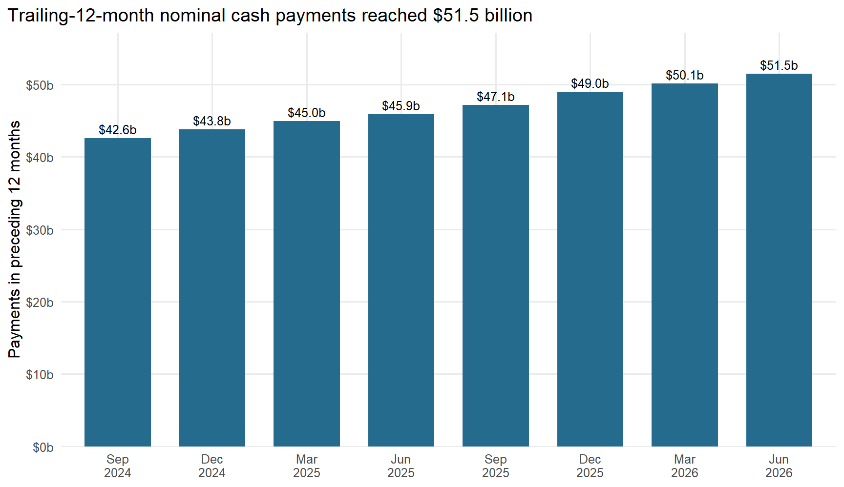
The first question is whether the latest payment increase was a one-period jump or part of a broader rise. Across the eight public releases from September 2024 to June 2026, the trailing-12-month nominal cash total increased each quarter.
## Nominal cash payments rose across every release shown
The payments files report the preceding 12 months at each reporting date. Each bar is therefore a rolling annual total, not a single quarter. Adjacent releases overlap by nine months, so the chart shows the path of annual payments rather than eight independent observations.
```{r}
#| label: payment-trend
#| fig-cap: "Trailing-12-month nominal cash-basis NDIS payments at each quarterly reporting date. Adjacent annual windows overlap by nine months."
#| fig-alt: "Eight bars rise from the September 2024 release through June 2026, when trailing-12-month nominal cash payments reach 51.5 billion dollars."
#| fig-width: 9
#| fig-height: 5.2
payment_trend_plot <- payment_trend |>
  mutate(period_label = format(report_date, "%b\n%Y"))

ggplot(payment_trend_plot, aes(factor(period_label, levels = period_label), total_payments)) +
  geom_col(fill = "#246b8e", width = 0.7) +
  geom_text(
    aes(label = dollar(total_payments, scale = 1e-9, suffix = "b", accuracy = 0.1)),
    vjust = -0.45,
    size = 3.4
  ) +
  scale_y_continuous(
    labels = label_dollar(scale = 1e-9, suffix = "b", accuracy = 1),
    limits = c(0, 56e9),
    expand = expansion(mult = c(0, 0.02))
  ) +
  labs(
    title = "Trailing-12-month nominal cash payments reached $51.5 billion",
    x = NULL,
    y = "Payments in preceding 12 months"
  )
```
The June-to-June comparison remains the cleanest year-on-year reading: payments increased by `r dollar(headline$payment_change, scale = 1e-9, suffix = " billion", accuracy = 0.1)`—`r percent(headline$payment_growth, accuracy = 0.1)`. The analysis makes no inflation adjustment, so this is not a measure of real service-volume growth.
## Participant count and the payment-to-participant ratio both rose
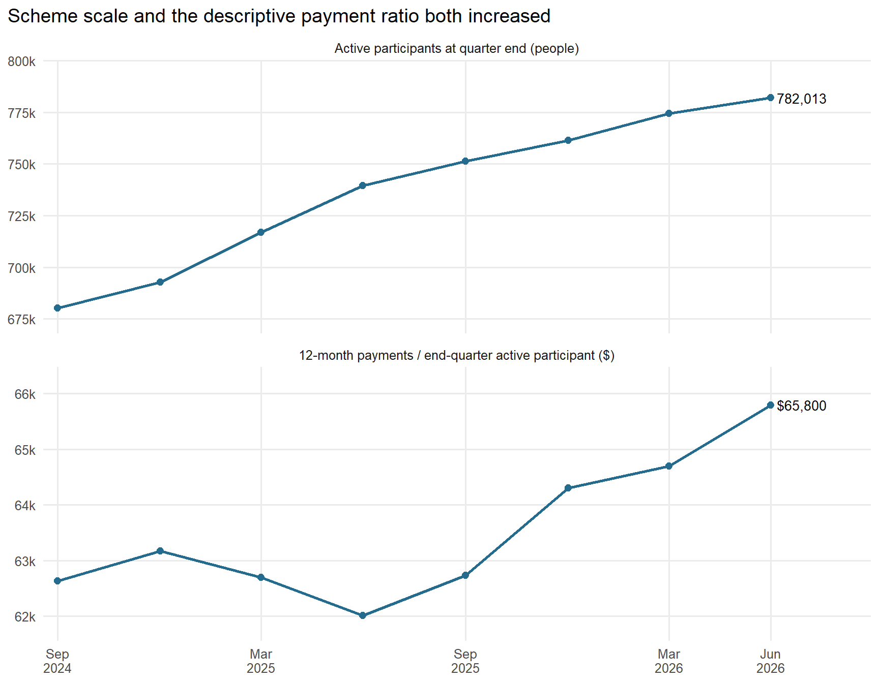
Active participants increased from `r comma(headline$participants_start)` at 30 June 2025 to `r comma(headline$participants_end)` at 30 June 2026. Over the same two reporting dates, trailing-12-month payments divided by the end-June active count rose from `r dollar(headline$payment_per_end_active_start, accuracy = 100)` to `r dollar(headline$payment_per_end_active_end, accuracy = 100)`.
That second measure is deliberately labelled as a ratio, not an average payment received by a participant. The numerator covers an entire year while the denominator is the active-participant stock on the final day. Entrants and exits during the year mean these two panels do not provide an exact decomposition of payment growth.
```{r}
#| label: participant-and-payment-ratio
#| fig-cap: "Active participants are a stock at each reporting date. The payment ratio divides the preceding 12 months of nominal cash payments by that end-quarter stock; it is useful context, not an exact average or causal decomposition."
#| fig-alt: "Two small-multiple line charts show active participants rising across the eight reporting dates and trailing-12-month payments per end-quarter active participant also rising."
#| fig-width: 9
#| fig-height: 7
participant_ratio_plot <- bind_rows(
  payment_trend |>
    transmute(
      report_date,
      metric = "Active participants at quarter end (people)",
      value = participants,
      latest_label = if_else(
        report_date == max(report_date),
        comma(participants, accuracy = 1),
        NA_character_
      )
    ),
  payment_trend |>
    transmute(
      report_date,
      metric = "12-month payments / end-quarter active participant ($)",
      value = payment_per_end_active_participant,
      latest_label = if_else(
        report_date == max(report_date),
        dollar(payment_per_end_active_participant, accuracy = 100),
        NA_character_
      )
    )
) |>
  mutate(metric = factor(
    metric,
    levels = c(
      "Active participants at quarter end (people)",
      "12-month payments / end-quarter active participant ($)"
    )
  ))

ggplot(participant_ratio_plot, aes(report_date, value)) +
  geom_line(colour = "#246b8e", linewidth = 1) +
  geom_point(colour = "#246b8e", size = 2.2) +
  geom_text(
    aes(label = latest_label),
    hjust = -0.12,
    size = 3.5,
    na.rm = TRUE
  ) +
  facet_wrap(~metric, scales = "free_y", ncol = 1) +
  scale_x_date(
    breaks = payment_trend$report_date[c(1, 3, 5, 7, 8)],
    labels = label_date("%b\n%Y"),
    expand = expansion(mult = c(0.02, 0.14))
  ) +
  scale_y_continuous(labels = label_number(scale = 1e-3, suffix = "k"), expand = expansion(mult = c(0.12, 0.18))) +
  labs(
    title = "Scheme scale and the descriptive payment ratio both increased",
    x = NULL,
    y = NULL
  )
```
## Most payment growth was in core supports
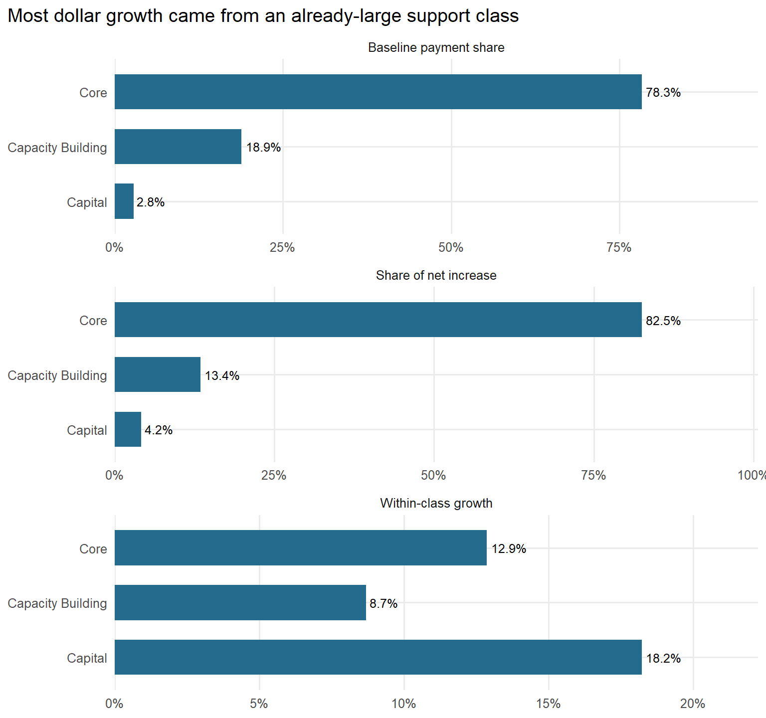
Core supports account for `r percent(core_change_share, accuracy = 1)` of the national increase. They rose by `r dollar(support_change_value("Core"), scale = 1e-9, suffix = " billion", accuracy = 0.1)`, compared with `r dollar(support_change_value("Capacity Building"), scale = 1e-9, suffix = " billion", accuracy = 0.1)` for capacity building and `r dollar(support_change_value("Capital"), scale = 1e-9, suffix = " billion", accuracy = 0.1)` for capital supports. Core also began as by far the largest class, so its dollar contribution should be read beside its baseline share and within-class growth.
```{r}
#| label: payments-by-support-class
#| fig-cap: "Baseline share, share of net payment growth and within-class growth for classified support classes, June 2025 to June 2026. Panel scales differ. Payments are nominal and cash-basis."
#| fig-alt: "Three-panel chart shows that Core was already the largest support class, supplied most of the net payment increase, and also grew within category."
#| fig-width: 8
#| fig-height: 7.5
support_plot <- support_change |>
  filter(support_class != "Missing") |>
  transmute(
    support_class,
    `Baseline payment share` = baseline_share,
    `Share of net increase` = growth_share,
    `Within-class growth` = within_growth
  ) |>
  pivot_longer(-support_class, names_to = "metric", values_to = "value") |>
  mutate(
    support_class = fct_relevel(support_class, "Core", "Capacity Building", "Capital") |> fct_rev(),
    metric = factor(metric, levels = c("Baseline payment share", "Share of net increase", "Within-class growth"))
  )

ggplot(support_plot, aes(value, support_class)) +
  geom_col(fill = "#246b8e", width = 0.64) +
  geom_text(aes(label = percent(value, accuracy = 0.1)), hjust = -0.12, size = 3.3) +
  facet_wrap(~metric, scales = "free_x", ncol = 1) +
  scale_x_continuous(labels = percent_format(accuracy = 1), expand = expansion(mult = c(0, 0.22))) +
  labs(
    title = "Most dollar growth came from an already-large support class",
    x = NULL, y = NULL
  ) +
  theme(panel.spacing.x = grid::unit(2, "lines"))
```
The June 2026 “Missing” support-class row is negative $3,000. It is retained in the national reconciliation but excluded from the chart as an apparent rounding or classification adjustment. The build separately checks that every classified support-class amount is non-negative.
## Published utilisation was 74%, versus 75%
The published average annualised committed support budget rose from `r dollar(headline$budget_start)` to `r dollar(headline$budget_end)` between the June reporting dates. That is a point-in-time plan-budget measure, not the average payment made during the preceding year, and the source rounds it to the nearest $1,000.
Utilisation has a third timing definition. The June 2026 figure covers supports delivered from October 2025 to March 2026 and paid by 30 June. It is a lagged six-month measure, not June-quarter utilisation and not the same window as the payment trend.
The source reports `r percent(headline$utilisation_end, accuracy = 1)` versus `r percent(headline$utilisation_start, accuracy = 1)` a year earlier. Because both figures are published as whole percentages, the public data support the reported comparison but not a precise estimate of the underlying change. The separately timed utilisation rate therefore cannot explain the payment increase.
## Most dollar growth came from already-large disability groups
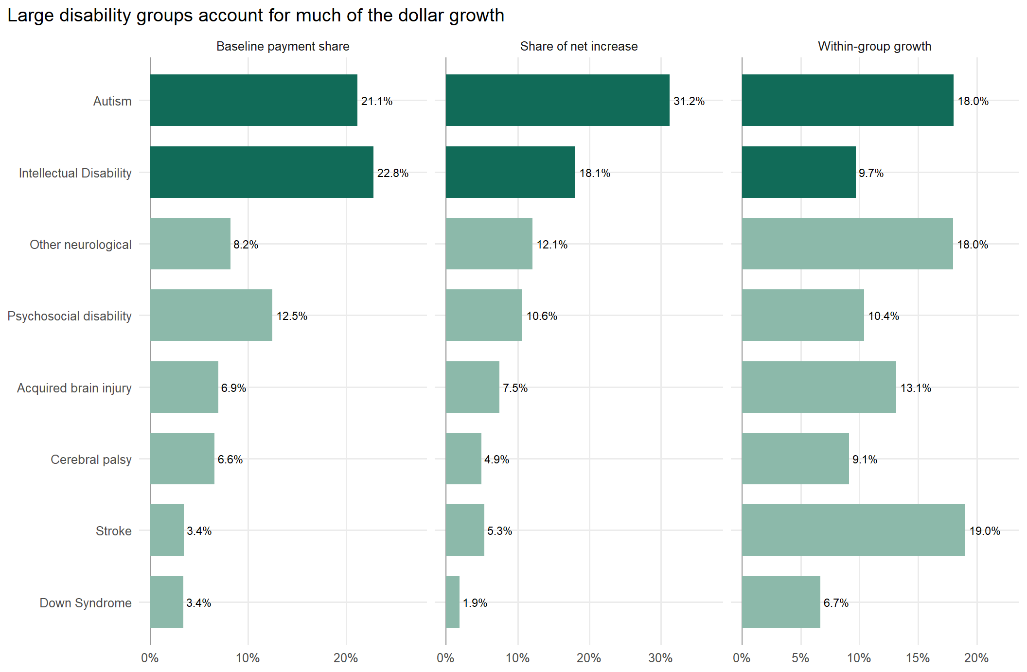
Autism and intellectual disability together accounted for `r percent(top_two_baseline_share, accuracy = 1)` of June 2025 payments and `r percent(top_two_share, accuracy = 1)` of the **net national increase**. Autism contributed `r dollar(autism_change, scale = 1e-9, suffix = " billion", accuracy = 0.01)` and intellectual disability `r dollar(intellectual_disability_change, scale = 1e-9, suffix = " billion", accuracy = 0.01)`; the five largest positive contributors account for `r percent(top_five_share, accuracy = 1)` of net growth.
This is an accounting contribution, not a causal finding. Dollar contributions partly reflect category size, so the chart shows baseline share and within-category growth beside share of the net increase. The totals combine changes in participant numbers, support mix, prices, payment timing and average payments.
```{r}
#| label: disability-contributions
#| fig-cap: "Baseline payment share, share of net payment growth and within-group growth for the eight largest classified primary-disability groups by June 2025 payments. Panel scales differ. Payments are nominal and cash-basis."
#| fig-alt: "Three-panel chart shows baseline payment share, share of net payment increase and within-group growth for the eight largest primary-disability payment groups. Autism and intellectual disability are large both at baseline and in dollar growth."
#| fig-width: 11
#| fig-height: 7.2
disability_plot_groups <- disability_change |>
  filter(!disability_group %in% c("Missing", "Suppression/reconciliation residual")) |>
  slice_max(`June 2025`, n = 8, with_ties = FALSE) |>
  pull(disability_group)

disability_plot <- disability_change |>
  filter(disability_group %in% disability_plot_groups) |>
  transmute(
    disability_group,
    `Baseline payment share` = baseline_share,
    `Share of net increase` = growth_share,
    `Within-group growth` = within_growth
  ) |>
  pivot_longer(-disability_group, names_to = "metric", values_to = "value") |>
  mutate(
    disability_group = recode(
      disability_group,
      "ABI" = "Acquired brain injury",
      "Other Neurological" = "Other neurological",
      "Cerebral Palsy" = "Cerebral palsy"
    ),
    disability_group = fct_reorder(disability_group, value),
    metric = factor(metric, levels = c("Baseline payment share", "Share of net increase", "Within-group growth")),
    emphasis = disability_group %in% c("Autism", "Intellectual Disability")
  )

ggplot(disability_plot, aes(value, disability_group, fill = emphasis)) +
  geom_vline(xintercept = 0, colour = "grey60") +
  geom_col(width = 0.72) +
  geom_text(aes(label = percent(value, accuracy = 0.1)), hjust = -0.12, size = 3.0) +
  facet_wrap(~metric, scales = "free_x", nrow = 1) +
  scale_x_continuous(labels = percent_format(accuracy = 1), expand = expansion(mult = c(0.05, 0.24))) +
  scale_fill_manual(values = c(`FALSE` = "#8cb9aa", `TRUE` = "#116b58"), guide = "none") +
  labs(title = "Large disability groups account for much of the dollar growth", x = NULL, y = NULL)
```
## What this changes about the story
The strongest public-data conclusion is descriptive and fairly narrow. Trailing-12-month nominal cash-basis payments rose across all eight quarterly releases shown and reached `r dollar(headline$payment_end, scale = 1e-9, suffix = " billion", accuracy = 0.1)` in June 2026. The end-quarter active-participant stock and the descriptive payment-to-active-participant ratio both rose, but their different windows prevent a causal decomposition. The separately timed utilisation rate was published as 74%, versus 75% a year earlier, while most dollar growth occurred in already-large categories.
The companion analysis asks a different question: [where reported participant outcomes changed after entry to the Scheme](../ndis-outcomes-spend-service-access/).
## Three-line takeaway
- Trailing-12-month nominal cash payments rose in every release shown and were `r percent(headline$payment_growth, accuracy = 0.1)` higher in June 2026 than a year earlier.
- Active participant numbers and payments divided by the end-period active count both rose; the latter is a stock/flow ratio, not an exact average or causal decomposition.
- The separately timed published utilisation rate was `r percent(headline$utilisation_end, accuracy = 1)`, versus `r percent(headline$utilisation_start, accuracy = 1)`, while most dollar growth occurred in categories that were already large.
## Appendix {#appendix}
::: {.callout-note collapse="true" title="Caveats, definitions and interpretation"}
The analysis does not identify why need, plan values or payments changed. The public extracts are rounded and suppress small cells, and their reporting windows differ. Primary-disability groups are administrative classifications, not fixed cohorts: composition can change as participants enter, leave, age and are reclassified. A participant-level causal model would require data these files do not contain.
Payments are nominal and cash-basis. This analysis does not adjust for inflation or estimate real service volume. Payment totals cover trailing-12-month windows; participant numbers and average annualised budgets are point-in-time measures; utilisation is a lagged six-month rate. The payment-to-end-active-participant measure divides a flow by a stock and is only a descriptive ratio. Entrants and exits during the year mean it is not the average payment received by a participant and cannot be used as a causal decomposition.
The earlier random-forest models and regional joins were removed because cross-sectional prediction cannot explain national payment growth from these aggregate files.
:::
::: {.callout-note collapse="true" title="Category accounting detail"}
```{r}
#| label: support-accounting-table
support_change |>
  transmute(
    `Support class` = support_class,
    `June 2025 payments` = dollar(`June 2025`, scale = 1e-9, suffix = "b", accuracy = 0.001),
    `June 2026 payments` = dollar(`June 2026`, scale = 1e-9, suffix = "b", accuracy = 0.001),
    `Baseline share` = percent(baseline_share, accuracy = 0.1),
    `Share of net increase` = percent(growth_share, accuracy = 0.1),
    `Within-class growth` = percent(within_growth, accuracy = 0.1)
  ) |>
  kable(align = c("l", "r", "r", "r", "r", "r"))
```
```{r}
#| label: disability-accounting-table
disability_change |>
  filter(!disability_group %in% c("Missing", "Suppression/reconciliation residual")) |>
  arrange(desc(`June 2025`)) |>
  transmute(
    `Primary disability group` = disability_group,
    `June 2025 payments` = dollar(`June 2025`, scale = 1e-9, suffix = "b", accuracy = 0.01),
    `June 2026 payments` = dollar(`June 2026`, scale = 1e-9, suffix = "b", accuracy = 0.01),
    `Baseline share` = percent(baseline_share, accuracy = 0.1),
    `Share of net increase` = percent(growth_share, accuracy = 0.1),
    `Within-group growth` = percent(within_growth, accuracy = 0.1)
  ) |>
  kable(align = c("l", "r", "r", "r", "r", "r"))
```
:::
::: {.callout-note collapse="true" title="Sources and reproducibility"}
The analysis uses the NDIA's [participant plan budget and utilisation datasets](https://dataresearch.ndis.gov.au/datasets/participant-datasets), [payments datasets](https://dataresearch.ndis.gov.au/datasets/payments-datasets), and their data-rules documents. The payment and participant trend uses quarterly releases from September 2024 to June 2026; the category and utilisation comparisons use the June 2025 and June 2026 releases. Each file is pinned by size and SHA-256 checksum in `sources.csv`; set `BLOG_REFRESH_DATA=true` to force a fresh download and checksum validation. In the registry, `release_date` records the downloadable asset's Last-Modified date.
```{r}
#| label: source-manifest
source_manifest |>
  transmute(
    source = dataset,
    source_revision_date = release_date,
    coverage_end,
    file = local_file,
    bytes = comma(bytes),
    sha256_prefix = substr(sha256, 1, 12)
  ) |>
  kable(col.names = c("Source", "Source/revision date", "Coverage end", "Cached file", "Bytes", "SHA-256 prefix"))
```
:::