---
title: "Did the 1 November 2025 Bulk Billing Changes Shift Access?"
description: "An early reproducible look at whether expanded GP bulk billing incentives changed access patterns by age, socioeconomic area, geography and PHN."
date: "2026-05-28"
categories: [medicare, bulk-billing, health-policy, australia]
author: "Aydin"
---
The 1 November 2025 bulk billing changes were designed to make it easier for general practices to bulk bill more patients. The narrowest measurable question is whether the share of GP attendances that were bulk billed moved after the change. The broader access question is harder: a higher bulk billing rate is not the same thing as more appointments, shorter waits or less delayed care.
This post treats access as two linked signals:
1. the GP bulk billing rate, which is the main outcome;
2. service-use and payment checks, so we do not confuse a billing-mix change with an access change.
The analysis is deliberately framed as an early signal. The policy began on 1 November 2025, the AIHW dashboard is updated quarterly, and AIHW treats the last 3 months of data as preliminary.
```{r}
#| label: setup
#| include: false
library(readr)
library(readxl)
library(dplyr)
library(tidyr)
library(ggplot2)
library(stringr)
library(lubridate)
library(purrr)
library(forcats)
library(broom)
library(scales)
library(knitr)
theme_set(theme_minimal(base_size = 12))
raw_dir <- file.path("data-raw")
dir.create(raw_dir, recursive = TRUE, showWarnings = FALSE)
policy_date <- as.Date("2025-11-01")
pre_start <- as.Date("2025-05-01")
pre_end <- as.Date("2025-10-01")
transition_quarter_date <- as.Date("2025-12-01")
clean_post_quarter_date <- as.Date("2026-03-01")
visit_model_start_quarter_date <- as.Date("2023-09-01")
source_urls <- list(
aihw_data = "https://www.aihw.gov.au/reports/medicare/medicare-bulk-billing-gp-attendances-monthly-data/data",
aihw_notes = "https://www.aihw.gov.au/reports/medicare/medicare-bulk-billing-gp-attendances-monthly-data/contents/technical-notes",
mbs_changes = "https://www.mbsonline.gov.au/internet/mbsonline/publishing.nsf/Content/Factsheet-Bulk%2BBilling%2BIncentives%2B%E2%80%93%2BChanges%2Bto%2BEligibility",
phn_quarterly = "https://www.health.gov.au/sites/default/files/2026-05/medicare-quarterly-statistics-bulk-billing-by-primary-health-network-march-quarter-2025-26.xlsx",
sa3_quarterly = "https://www.health.gov.au/sites/default/files/2026-05/medicare-quarterly-statistics-statistical-area-sa3-summary-march-quarter-2025-26.xlsx",
mmm_quarterly = "https://www.health.gov.au/sites/default/files/2026-05/medicare-quarterly-statistics-modified-monash-model-locations-march-quarter-2025-26.xlsx",
primary_care_service_type = "https://www.health.gov.au/sites/default/files/2026-05/medicare-quarterly-statistics-primary-care-service-type-summary-march-quarter-2025-26.xlsx",
phn_lga = "https://www.health.gov.au/sites/default/files/2024-03/primary-health-networks-phn-2023-local-government-areas-2021.xlsx",
mmm_feature = "https://services5.arcgis.com/OvOcYIrJnM97ABBA/ArcGIS/rest/services/Modified_Monash_Model_2019/FeatureServer/0"
)
clean_names <- function(x) {
x |>
str_to_lower() |>
str_replace_all("&", "and") |>
str_replace_all("[^a-z0-9]+", "_") |>
str_replace_all("^_|_$", "")
}
clean_df <- function(x) {
names(x) <- clean_names(names(x))
x
}
first_col <- function(data, pattern, required = TRUE) {
hit <- names(data)[str_detect(names(data), regex(pattern, ignore_case = TRUE))]
if (length(hit) == 0) {
if (required) stop("Could not find column matching: ", pattern)
return(NA_character_)
}
hit[[1]]
}
as_number <- function(x) {
if (is.numeric(x)) return(x)
parse_number(as.character(x), na = c("", "NA", "n/a", "-", "%null%"))
}
safe_mean <- function(x) {
x <- x[is.finite(x)]
if (length(x) == 0) return(NA_real_)
mean(x)
}
safe_lm_slope <- function(data) {
if (nrow(data) < 6 || n_distinct(data$service_month) < 6) return(NA_real_)
tidy(lm(bulk_billing_rate ~ month_index, data = data)) |>
filter(term == "month_index") |>
pull(estimate)
}
quarter_to_date <- function(x) {
fy_start <- as.integer(str_extract(x, "^\\d{4}"))
quarter <- as.integer(str_match(x, "Q([1-4])")[, 2])
month <- case_when(
quarter == 1 ~ 9L,
quarter == 2 ~ 12L,
quarter == 3 ~ 3L,
quarter == 4 ~ 6L,
TRUE ~ NA_integer_
)
year <- if_else(quarter %in% c(1L, 2L), fy_start, fy_start + 1L)
as.Date(sprintf("%04d-%02d-01", year, month))
}
weighted_rate <- function(numerator, denominator) {
total_denominator <- sum(denominator, na.rm = TRUE)
if (!is.finite(total_denominator) || total_denominator == 0) return(NA_real_)
sum(numerator, na.rm = TRUE) / total_denominator
}
format_model_estimate <- function(estimate, outcome_type) {
case_when(
outcome_type == "log" ~ percent(exp(estimate) - 1, accuracy = 0.1),
outcome_type == "rate" ~ percent(estimate, accuracy = 0.01),
outcome_type == "dollar" ~ dollar(estimate, accuracy = 0.01),
TRUE ~ as.character(round(estimate, 3))
)
}
download_if_missing <- function(url, path) {
if (!file.exists(path)) {
ok <- tryCatch({
download.file(url, path, mode = "wb", quiet = TRUE, timeout = 180)
TRUE
}, error = function(e) FALSE)
if (!ok && nzchar(Sys.which("curl"))) {
status <- system2(
"curl",
c("-L", "--fail", "--retry", "3", "--connect-timeout", "20", "--max-time", "180", "-o", shQuote(path), shQuote(url)),
stdout = TRUE,
stderr = TRUE
)
ok <- file.exists(path)
if (!ok) warning(paste(status, collapse = "\n"))
}
if (!ok) stop("Could not download source file: ", url)
}
path
}
ensure_aihw_tableau <- function(refresh = FALSE) {
expected <- file.path(
raw_dir,
paste0(
"aihw_tableau_",
c("national", "age", "seifa", "benefits", "latest_lga_map"),
".csv"
)
)
if (refresh || any(!file.exists(expected))) {
script <- if (file.exists("tableau_export.py")) {
"tableau_export.py"
} else {
file.path("posts", "bulk-billing-changes-impact", "tableau_export.py")
}
if (!file.exists(script)) stop("Missing Tableau extractor: ", script)
python_cmd <- if (.Platform$OS.type == "windows") "py" else "python3"
python_args <- if (.Platform$OS.type == "windows") {
c("-3", shQuote(script), "--out-dir", shQuote(normalizePath(raw_dir, winslash = "/")))
} else {
c(shQuote(script), "--out-dir", shQuote(normalizePath(raw_dir, winslash = "/")))
}
status <- system2(
python_cmd,
python_args,
stdout = TRUE,
stderr = TRUE
)
if (!all(file.exists(expected))) {
stop("AIHW Tableau extraction did not create all expected files:\n", paste(status, collapse = "\n"))
}
}
invisible(expected)
}
read_tableau <- function(label) {
read_csv(file.path(raw_dir, paste0("aihw_tableau_", label, ".csv")), show_col_types = FALSE) |>
clean_df()
}
standardise_rate_sheet <- function(data, dimension_col = NULL, dimension_name = "All") {
value_col <- first_col(data, "^sum_pivot_field_values_value$")
month_col <- first_col(data, "^month_service_month_value$")
state_col <- first_col(data, "^attr_state1_alias$", required = FALSE)
type_col <- first_col(data, "^type_alias$", required = FALSE)
out <- data |>
transmute(
service_month = as.Date(.data[[month_col]]),
state = if (!is.na(state_col)) .data[[state_col]] else "Australia",
dimension = dimension_name,
group = if (is.null(dimension_col)) "All patients" else as.character(.data[[dimension_col]]),
type = if (!is.na(type_col)) .data[[type_col]] else "Total",
bulk_billing_rate = as.numeric(.data[[value_col]])
) |>
filter(!is.na(service_month), type == "Total", is.finite(bulk_billing_rate)) |>
distinct()
out
}
extract_latest <- function(data, value_col = "bulk_billing_rate") {
data |>
filter(service_month == max(service_month, na.rm = TRUE)) |>
arrange(desc(.data[[value_col]]))
}
window_compare <- function(data) {
data |>
mutate(window = case_when(
service_month >= pre_start & service_month <= pre_end ~ "May-Oct 2025",
service_month >= policy_date ~ "Nov 2025 onward",
TRUE ~ NA_character_
)) |>
filter(!is.na(window)) |>
group_by(dimension, group, window) |>
summarise(rate = safe_mean(bulk_billing_rate), months = n_distinct(service_month), .groups = "drop") |>
pivot_wider(names_from = window, values_from = c(rate, months)) |>
mutate(change = `rate_Nov 2025 onward` - `rate_May-Oct 2025`) |>
arrange(desc(abs(change)))
}
```
```{r}
#| label: load-data
ensure_aihw_tableau(refresh = FALSE)

manifest <- read_csv(file.path(raw_dir, "aihw_tableau_manifest.csv"), show_col_types = FALSE)

national <- read_tableau("national") |>
  standardise_rate_sheet() |>
  mutate(month_index = as.integer(interval(min(service_month), service_month) %/% months(1)))

age_rates <- read_tableau("age") |>
  standardise_rate_sheet("age_group_series_alias", "Age group") |>
  mutate(group = str_replace(group, " - ", "-"))

seifa_rates <- read_tableau("seifa") |>
  standardise_rate_sheet("seifa_series_alias", "Socioeconomic quintile")

benefits_raw <- read_tableau("benefits")
benefits <- benefits_raw |>
  transmute(
    service_month = as.Date(.data[[first_col(benefits_raw, "^month_service_month_value$")]]),
    series = .data[[first_col(benefits_raw, "^chart_4_series_alias$")]],
    value = as.numeric(.data[[first_col(benefits_raw, "^sum_pivot_field_values_value$")]])
  ) |>
  filter(!is.na(service_month), is.finite(value), !is.na(series)) |>
  distinct()

lga_latest <- read_tableau("latest_lga_map") |>
  transmute(
    state = state1_alias,
    lga_code = as.integer(lga_code21_alias),
    lga_name = attr_lga_name_alias,
    latest_bulk_billing_rate = as_number(sum_pivot_field_values_copy_alias),
    remoteness_area = attr_main_ra_alias,
    seifa_quintile = as.integer(attr_main_seifa_alias)
  ) |>
  filter(is.finite(latest_bulk_billing_rate), !is.na(lga_code))

phn_path <- download_if_missing(source_urls$phn_quarterly, file.path(raw_dir, "phn_bulk_billing.xlsx"))
sa3_path <- download_if_missing(source_urls$sa3_quarterly, file.path(raw_dir, "sa3_quarterly.xlsx"))
mmm_path <- download_if_missing(source_urls$mmm_quarterly, file.path(raw_dir, "mmm_quarterly.xlsx"))
pcst_path <- download_if_missing(source_urls$primary_care_service_type, file.path(raw_dir, "primary_care_service_type.xlsx"))
phn_lga_path <- download_if_missing(source_urls$phn_lga, file.path(raw_dir, "phn_lga_concordance.xlsx"))

phn_quarterly <- read_excel(phn_path, sheet = "By BTOS and PHN", skip = 4) |>
  clean_df() |>
  transmute(
    state,
    phn = primary_health_network,
    quarter,
    service_type = broad_type_of_service,
    phn_bulk_billing_rate = as.numeric(mbs_bulk_billing_rate)
  ) |>
  filter(service_type == "Total GP Non-Referred Attendances", !is.na(phn_bulk_billing_rate))

phn_age <- read_excel(phn_path, sheet = "GP NRA by PHN and Age Group", skip = 4) |>
  clean_df() |>
  select(state, phn = primary_health_network, quarter, contains("bulk_billing_rate")) |>
  pivot_longer(contains("bulk_billing_rate"), names_to = "age_group", values_to = "bulk_billing_rate") |>
  mutate(
    age_group = case_when(
      str_detect(age_group, "under_16") ~ "0-15",
      str_detect(age_group, "16_to_64") ~ "16-64",
      str_detect(age_group, "65") ~ "65+",
      str_detect(age_group, "all_ages") ~ "All ages",
      TRUE ~ age_group
    ),
    bulk_billing_rate = as.numeric(bulk_billing_rate)
  ) |>
  filter(!is.na(bulk_billing_rate))

sa3_visits_raw <- read_excel(sa3_path, sheet = "GP NRA by SA3", skip = 4) |>
  clean_df()

sa3_visits <- sa3_visits_raw |>
  transmute(
    state,
    sa3 = sa3,
    quarter,
    quarter_date = quarter_to_date(quarter),
    service_type = broad_type_of_service,
    services = as.numeric(services),
    benefits = as.numeric(benefits),
    bulk_billed_services = as.numeric(bulk_billed_services),
    patient_billed_services = as.numeric(patient_billed_services),
    bulk_billing_rate = as.numeric(mbs_bulk_billing_rate),
    avg_patient_contribution_patient_billed = as.numeric(avg_patient_contribution_per_service_out_of_hospital_patient_billed),
    avg_patient_contribution_total = as.numeric(avg_patient_contribution_per_service_out_of_hospital_total)
  ) |>
  filter(
    service_type == "Total GP Non-Referred Attendances",
    !is.na(quarter_date),
    is.finite(services),
    services > 0,
    !sa3 %in% c("Australia", state),
    !str_detect(state, regex("unknown|other territories", ignore_case = TRUE)),
    !str_detect(sa3, regex("^unknown|unknown state", ignore_case = TRUE))
  ) |>
  mutate(
    sa3_key = paste(state, sa3, sep = " - "),
    quarter_status = case_when(
      quarter_date < transition_quarter_date ~ "Pre-policy",
      quarter_date == transition_quarter_date ~ "Transition quarter",
      quarter_date >= clean_post_quarter_date ~ "Clean post-policy",
      TRUE ~ NA_character_
    )
  )

sa3_exposure <- sa3_visits |>
  filter(
    quarter_date >= max(quarter_date[quarter_date < transition_quarter_date], na.rm = TRUE) %m-% months(9),
    quarter_date < transition_quarter_date
  ) |>
  group_by(sa3_key) |>
  summarise(
    baseline_quarters = n_distinct(quarter_date),
    baseline_services = mean(services, na.rm = TRUE),
    pre_policy_bulk_billing_rate = weighted_rate(bulk_billed_services, services),
    pre_policy_patient_contribution = weighted.mean(
      avg_patient_contribution_patient_billed,
      w = patient_billed_services,
      na.rm = TRUE
    ),
    .groups = "drop"
  ) |>
  mutate(
    pre_policy_non_bulk_billed_share = 1 - pre_policy_bulk_billing_rate,
    pre_policy_gap_10pp = pre_policy_non_bulk_billed_share / 0.1
  )

sa3_panel <- sa3_visits |>
  left_join(sa3_exposure, by = "sa3_key") |>
  mutate(
    log_services = log1p(services),
    clean_post_policy = quarter_date >= clean_post_quarter_date,
    exposure_band = cut(
      pre_policy_non_bulk_billed_share,
      breaks = quantile(pre_policy_non_bulk_billed_share, probs = c(0, 1 / 3, 2 / 3, 1), na.rm = TRUE),
      include.lowest = TRUE,
      labels = c("Lower room to move", "Middle", "Higher room to move")
    ),
    rate_check = bulk_billed_services / services,
    rate_difference = bulk_billing_rate - rate_check
  ) |>
  filter(
    is.finite(pre_policy_gap_10pp),
    is.finite(baseline_services),
    baseline_quarters == 4
  )

mmm_visits <- read_excel(mmm_path, sheet = "All Services", skip = 4) |>
  clean_df() |>
  transmute(
    modified_monash = modified_monash_group,
    quarter,
    quarter_date = quarter_to_date(quarter),
    service_type = broad_type_of_service,
    services = as.numeric(services),
    bulk_billed_services = as.numeric(bulk_billed_services),
    patient_billed_services = as.numeric(patient_billed_services),
    bulk_billing_rate = as.numeric(mbs_bulk_billing_rate)
  ) |>
  filter(
    service_type == "Total GP Non-Referred Attendances",
    !is.na(quarter_date),
    is.finite(services),
    services > 0,
    !modified_monash %in% c("Australia")
  ) |>
  mutate(
    quarter_status = case_when(
      quarter_date < transition_quarter_date ~ "Pre-policy",
      quarter_date == transition_quarter_date ~ "Transition quarter",
      quarter_date >= clean_post_quarter_date ~ "Clean post-policy",
      TRUE ~ NA_character_
    )
  )

pcst_quarters <- read_excel(pcst_path, sheet = "State", skip = 4) |>
  clean_df() |>
  transmute(
    quarter,
    quarter_date = quarter_to_date(quarter),
    service_type = broad_type_of_service,
    primary_care_service_type,
    services = as.numeric(services)
  ) |>
  filter(!is.na(quarter_date), service_type == "Total GP Non-Referred Attendances")

phn_lga <- read_excel(phn_lga_path) |>
  clean_df() |>
  transmute(
    lga_code = as.integer(lga_code_2021),
    lga_name = lga_name_2021,
    phn_code = phn_code_2023,
    phn = phn_name_2023,
    ratio = as.numeric(ratio_from_to)
  )

lga_phn_latest <- lga_latest |>
  left_join(phn_lga, by = "lga_code", suffix = c("", "_phn")) |>
  group_by(phn) |>
  summarise(
    lgas = n_distinct(lga_code),
    latest_lga_mean_rate = weighted.mean(latest_bulk_billing_rate, w = coalesce(ratio, 1), na.rm = TRUE),
    .groups = "drop"
  ) |>
  filter(!is.na(phn))
```
## Source Audit
The AIHW monthly dashboard is the main source because it is dated by month of service and has the policy date built into the time series. The Department's PHN workbook is added as a quarterly cross-check because it has current PHN and age information, but it is not identical to the AIHW dashboard.
```{r}
#| label: audit-table
audit <- tibble(
  source = c(
    "AIHW Tableau monthly dashboard",
    "Department quarterly PHN workbook",
    "Department quarterly SA3 workbook",
    "Department quarterly MMM workbook",
    "Department primary care service type workbook",
    "PHN 2023 to LGA 2021 concordance",
    "Modified Monash Model 2019 feature service"
  ),
  used_for = c(
    "Monthly national, age, SEIFA, benefits and latest LGA map",
    "Quarterly PHN and PHN by age cross-check",
    "Quarterly SA3 GP visit-volume panel",
    "Quarterly Modified Monash visit-volume cross-check",
    "Primary care service type source audit",
    "Approximate latest LGA-to-PHN grouping",
    "Documented as the correct MMM source; not spatially joined in this render"
  ),
  latest_period = c(
    format(max(national$service_month), "%B %Y"),
    phn_quarterly$quarter[[1]],
    sa3_panel |>
      filter(quarter_date == max(quarter_date, na.rm = TRUE)) |>
      pull(quarter) |>
      first(),
    mmm_visits |>
      filter(quarter_date == max(quarter_date, na.rm = TRUE)) |>
      pull(quarter) |>
      first(),
    pcst_quarters |>
      filter(quarter_date == max(quarter_date, na.rm = TRUE)) |>
      pull(quarter) |>
      first(),
    "2021 LGA to 2023 PHN",
    "2019 MMM polygons"
  ),
  caveat = c(
    "Last 3 months are preliminary and may revise",
    "Quarterly and processed-date style statistics may differ from AIHW",
    "December quarter 2025 is a transition quarter, not a clean post-policy period",
    "Coarser than SA3 but directly reports Modified Monash categories",
    "Used for source triangulation, not the main model",
    "Latest LGA means are not attendance-weighted",
    "A faithful MMM join needs spatial or mesh-block concordance work"
  )
)

audit |> kable()
```
```{r}
#| label: source-manifest
manifest |> kable()
```
The extract found `r n_distinct(national$service_month)` monthly observations from `r format(min(national$service_month), "%B %Y")` to `r format(max(national$service_month), "%B %Y")`. There are `r sum(national$service_month < policy_date & national$service_month >= pre_start)` months in the immediate pre-window and `r sum(national$service_month >= policy_date)` months after the policy start.
## National Signal
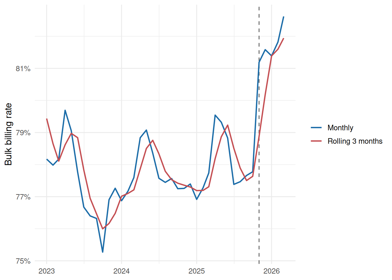
The national monthly rate is the cleanest first test. A one-off step after November is suggestive, but the stronger signal is a step that is larger than the pre-existing trend and is visible in the 3-month average.
```{r}
#| label: national-before-after
national_summary <- window_compare(national) |>
  mutate(
    across(starts_with("rate"), \(x) percent(x, accuracy = 0.1)),
    change = percent(change, accuracy = 0.1)
  )

national_summary |> kable()
```
```{r}
#| label: national-trend
#| fig-cap: "National GP bulk billing rate, with a 3-month rolling average."
national_plot <- national |>
  arrange(service_month) |>
  mutate(
    rolling_3_month = (bulk_billing_rate + lag(bulk_billing_rate, 1) + lag(bulk_billing_rate, 2)) / 3
  ) |>
  filter(service_month >= as.Date("2023-01-01")) |>
  pivot_longer(c(bulk_billing_rate, rolling_3_month), names_to = "measure", values_to = "rate")

ggplot(national_plot, aes(service_month, rate, colour = measure)) +
  geom_vline(xintercept = policy_date, linetype = "dashed", colour = "grey40") +
  geom_line(linewidth = 0.8, na.rm = TRUE) +
  scale_y_continuous(labels = percent) +
  scale_colour_manual(
    values = c(bulk_billing_rate = "#1b6ca8", rolling_3_month = "#c44e52"),
    labels = c(bulk_billing_rate = "Monthly", rolling_3_month = "Rolling 3 months")
  ) +
  labs(x = NULL, y = "Bulk billing rate", colour = NULL)
```
```{r}
#| label: national-event-model
model_data <- national |>
  filter(service_month >= as.Date("2023-01-01")) |>
  mutate(
    post = service_month >= policy_date,
    months_since_policy = pmax(0, as.integer(interval(policy_date, service_month) %/% months(1))),
    month_index = as.integer(interval(min(service_month), service_month) %/% months(1))
  )

its_model <- lm(bulk_billing_rate ~ month_index + post + months_since_policy, data = model_data)

tidy(its_model, conf.int = TRUE) |>
  mutate(
    estimate = percent(estimate, accuracy = 0.01),
    conf.low = percent(conf.low, accuracy = 0.01),
    conf.high = percent(conf.high, accuracy = 0.01)
  ) |>
  kable()
```
The `postTRUE` coefficient is the immediate step after November 2025, after allowing for a linear pre/post time trend. This is useful as a screening estimate, not as a final causal estimate.
## Who Moved?
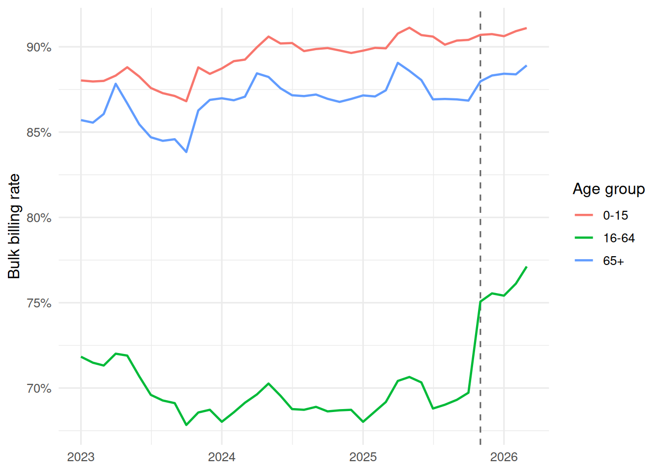
The policy should matter most for patients who were not already covered by the old child/concession-heavy incentive structure. In the public AIHW age bands, that makes `16-64` the group to watch.
```{r}
#| label: age-before-after
age_compare <- window_compare(age_rates) |>
  mutate(
    across(starts_with("rate"), \(x) percent(x, accuracy = 0.1)),
    change = percent(change, accuracy = 0.1)
  )

age_compare |> kable()
```
```{r}
#| label: age-trend
#| fig-cap: "Bulk billing rates by age group."
age_rates |>
  filter(service_month >= as.Date("2023-01-01")) |>
  ggplot(aes(service_month, bulk_billing_rate, colour = group)) +
  geom_vline(xintercept = policy_date, linetype = "dashed", colour = "grey40") +
  geom_line(linewidth = 0.8) +
  scale_y_continuous(labels = percent) +
  labs(x = NULL, y = "Bulk billing rate", colour = "Age group")
```
```{r}
#| label: seifa-before-after
seifa_compare <- window_compare(seifa_rates) |>
  mutate(
    across(starts_with("rate"), \(x) percent(x, accuracy = 0.1)),
    change = percent(change, accuracy = 0.1)
  )

seifa_compare |> kable()
```
```{r}
#| label: seifa-trend
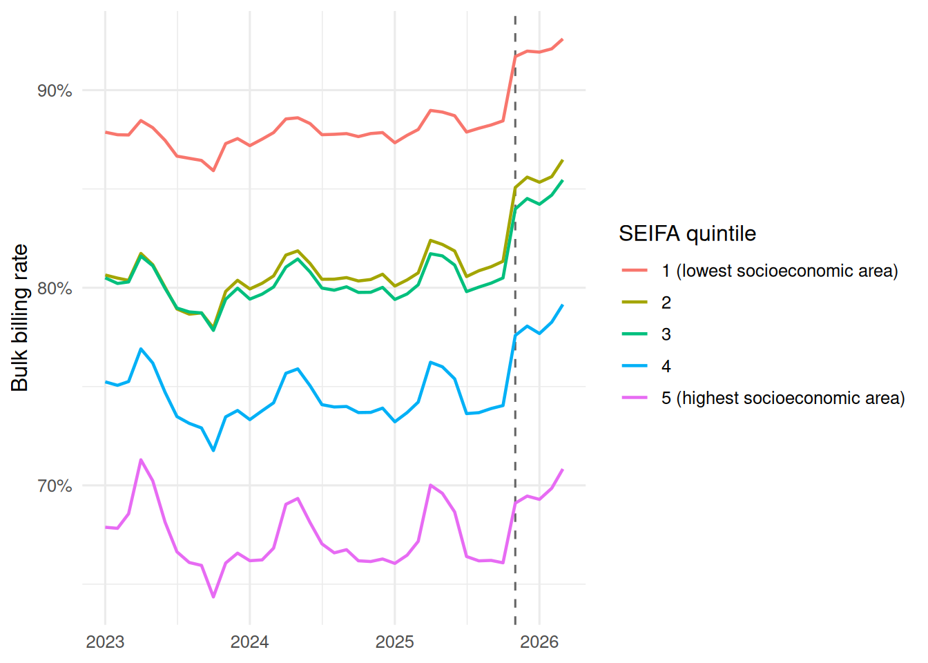
#| fig-cap: "Bulk billing rates by socioeconomic quintile."
seifa_rates |>
  filter(service_month >= as.Date("2023-01-01")) |>
  mutate(group = fct_relevel(group, "1 (lowest socioeconomic area)", "2", "3", "4", "5 (highest socioeconomic area)")) |>
  ggplot(aes(service_month, bulk_billing_rate, colour = group)) +
  geom_vline(xintercept = policy_date, linetype = "dashed", colour = "grey40") +
  geom_line(linewidth = 0.8) +
  scale_y_continuous(labels = percent) +
  labs(x = NULL, y = "Bulk billing rate", colour = "SEIFA quintile")
```
## Payment Check
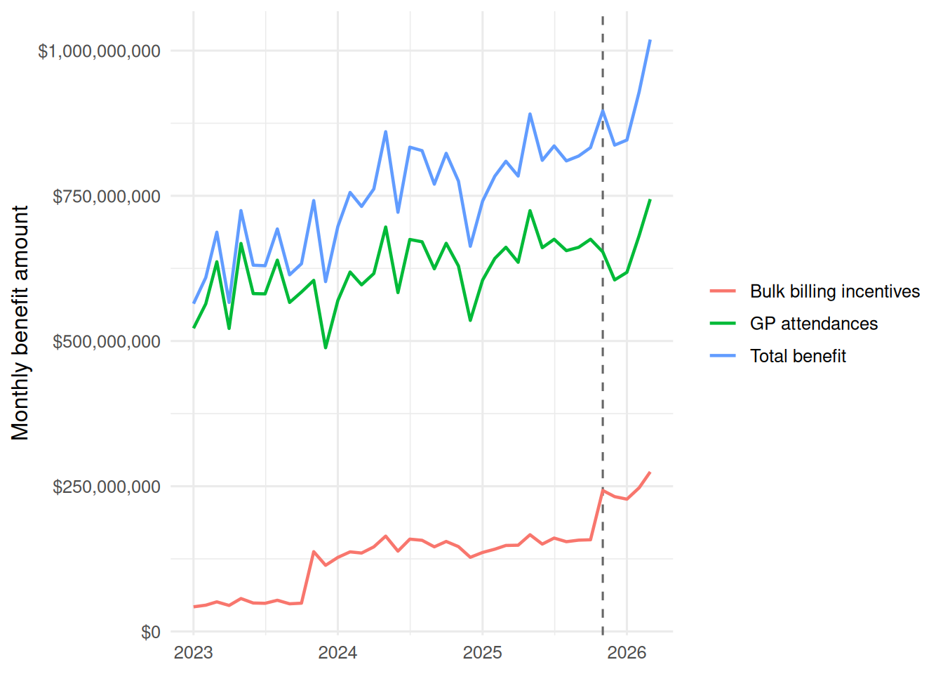
AIHW's benefits measure includes Medicare benefits for bulk billed GP attendances and the matched bulk billing incentive items. It does not include the separate Bulk Billing Practice Incentive Program payments.
```{r}
#| label: benefits-check
#| fig-cap: "Bulk billed GP attendance benefits and related bulk billing incentives."
benefits |>
  filter(service_month >= as.Date("2023-01-01")) |>
  ggplot(aes(service_month, value, colour = series)) +
  geom_vline(xintercept = policy_date, linetype = "dashed", colour = "grey40") +
  geom_line(linewidth = 0.8) +
  scale_y_continuous(labels = dollar) +
  labs(x = NULL, y = "Monthly benefit amount", colour = NULL)
```
```{r}
#| label: incentive-share
benefit_wide <- benefits |>
  filter(service_month >= as.Date("2025-05-01")) |>
  pivot_wider(names_from = series, values_from = value)

if (all(c("Bulk billing incentives", "Total benefit") %in% names(benefit_wide))) {
  benefit_wide |>
    transmute(
      service_month,
      incentive_share = `Bulk billing incentives` / `Total benefit`
    ) |>
    arrange(service_month) |>
    mutate(incentive_share = percent(incentive_share, accuracy = 0.1)) |>
    kable()
} else {
  tibble(note = "The expected incentive and total benefit series were not both present in the Tableau export.") |>
    kable()
}
```
## Geography
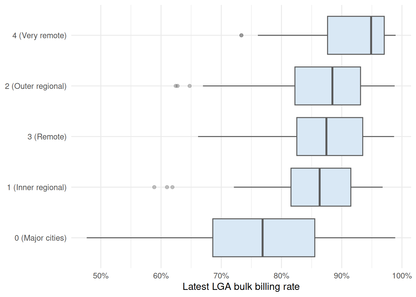
The AIHW dashboard gives a latest-month LGA map. That is not enough for an LGA-level before/after model, but it is enough to see where the current access surface is high or low. The PHN grouping below is an approximate LGA-to-PHN summary of latest LGA rates, not an attendance-weighted PHN statistic.
```{r}
#| label: lga-latest-extremes
bind_rows(
  lga_latest |>
    arrange(latest_bulk_billing_rate) |>
    slice_head(n = 10) |>
    mutate(rank_type = "Lowest latest LGA rates"),
  lga_latest |>
    arrange(desc(latest_bulk_billing_rate)) |>
    slice_head(n = 10) |>
    mutate(rank_type = "Highest latest LGA rates")
) |>
  transmute(
    rank_type,
    state,
    lga_name,
    remoteness_area,
    seifa_quintile,
    latest_bulk_billing_rate = percent(latest_bulk_billing_rate, accuracy = 0.1)
  ) |>
  kable()
```
```{r}
#| label: lga-remoteness
#| fig-cap: "Latest LGA bulk billing rates by AIHW remoteness field."
lga_latest |>
  filter(!is.na(remoteness_area)) |>
  ggplot(aes(fct_reorder(remoteness_area, latest_bulk_billing_rate, .fun = median, na.rm = TRUE), latest_bulk_billing_rate)) +
  geom_boxplot(fill = "#d9e8f5", colour = "grey35", outlier.alpha = 0.35) +
  coord_flip() +
  scale_y_continuous(labels = percent) +
  labs(x = NULL, y = "Latest LGA bulk billing rate")
```
```{r}
#| label: phn-lga-latest
lga_phn_latest |>
  arrange(latest_lga_mean_rate) |>
  slice_head(n = 15) |>
  mutate(latest_lga_mean_rate = percent(latest_lga_mean_rate, accuracy = 0.1)) |>
  kable()
```
The Modified Monash Model source is available as a polygon feature service, but this render does not force a low-quality LGA-only MMM approximation. A proper MMM join should use a spatial intersection or a finer ABS geography concordance, then aggregate to the patient geography used by the Medicare data.
## PHN Cross-Check
The Department's PHN workbook is quarterly. It is useful as a second view of whether the post-policy shift is visible across PHNs, and whether the working-age pattern appears there too.
```{r}
#| label: phn-quarterly-summary
phn_quarterly |>
  filter(phn %in% c("Australia", "NSW", "VIC", "QLD", "SA", "WA", "TAS", "ACT", "NT")) |>
  arrange(quarter, state, phn) |>
  tail(20) |>
  mutate(phn_bulk_billing_rate = percent(phn_bulk_billing_rate, accuracy = 0.1)) |>
  kable()
```
```{r}
#| label: phn-latest
latest_phn_quarter <- phn_quarterly$quarter[[1]]

phn_quarterly |>
  filter(quarter == latest_phn_quarter, !phn %in% c("Australia", state)) |>
  arrange(phn_bulk_billing_rate) |>
  slice_head(n = 15) |>
  transmute(
    quarter,
    state,
    phn,
    phn_bulk_billing_rate = percent(phn_bulk_billing_rate, accuracy = 0.1)
  ) |>
  kable()
```
```{r}
#| label: phn-age-latest
phn_age |>
  filter(quarter == latest_phn_quarter, phn == "Australia", age_group != "All ages") |>
  transmute(
    quarter,
    age_group,
    bulk_billing_rate = percent(bulk_billing_rate, accuracy = 0.1)
  ) |>
  kable()
```
## Visit Access
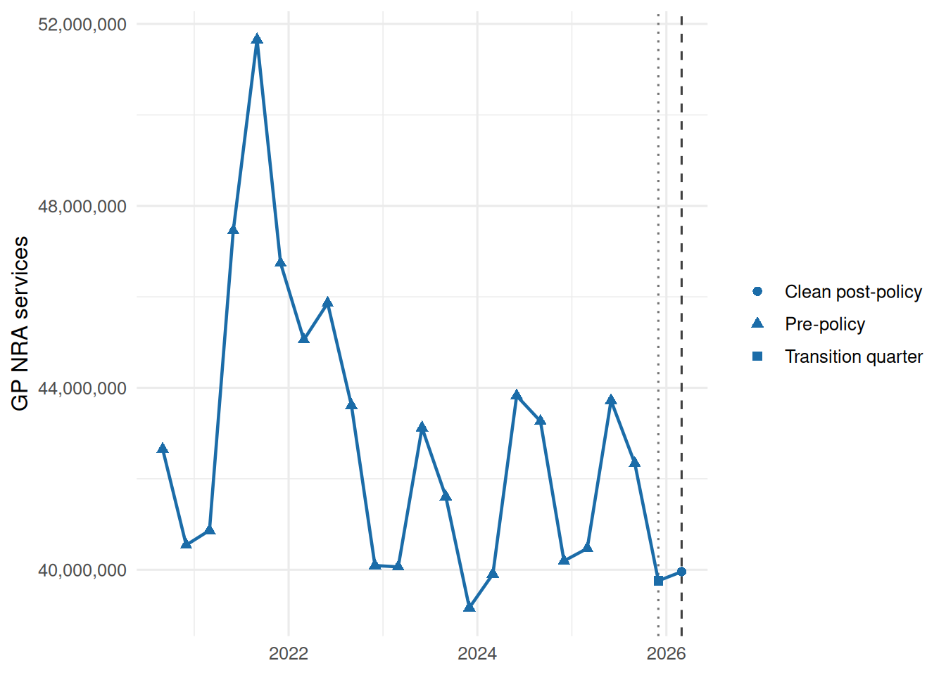
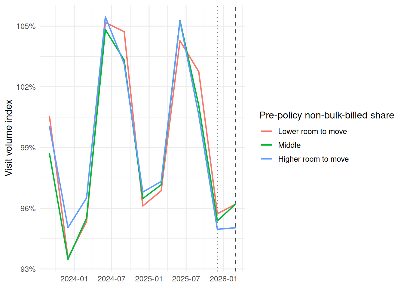
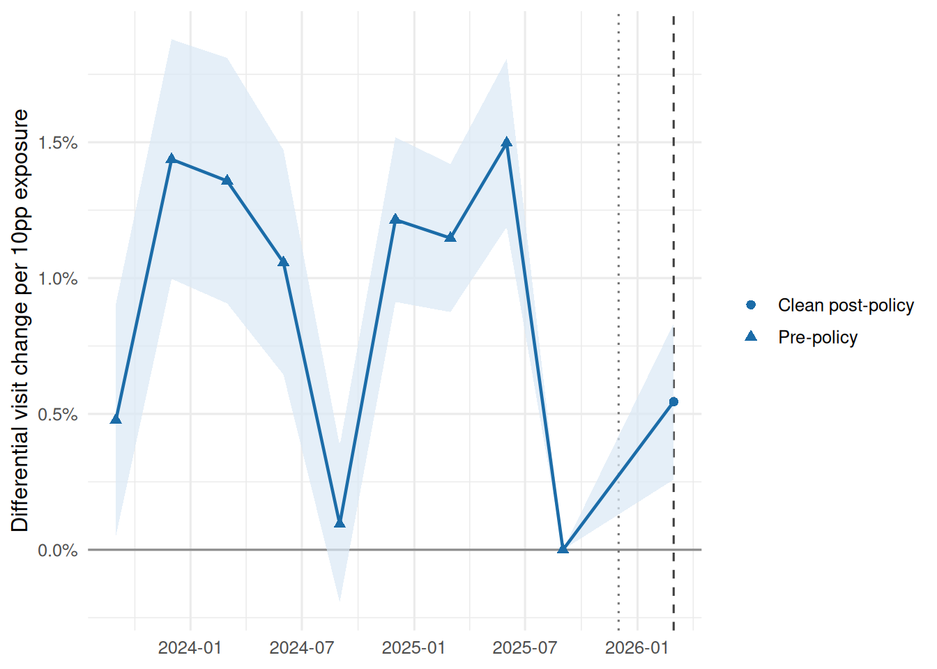
The next test is stricter: did areas with more room for the incentive to shift billing also see more GP attendances? For this, the lowest-level public panel in the current official releases is SA3 by quarter. The December quarter 2025 is mixed, because October was pre-policy and November-December were post-policy, so it is labelled as a transition quarter and excluded from the fixed-effects model.
```{r}
#| label: visit-access-audit
exposure_baseline_quarters <- sa3_panel |>
  filter(quarter_date < transition_quarter_date) |>
  distinct(quarter, quarter_date) |>
  arrange(desc(quarter_date)) |>
  slice_head(n = 4) |>
  arrange(quarter_date)

visit_access_audit <- tibble(
  metric = c(
    "Latest SA3 quarter",
    "Usable pre-policy quarters",
    "Exposure baseline window",
    "Transition quarter",
    "Visit model window starts",
    "Clean post-policy quarters",
    "SA3s in model panel",
    "Rows with missing model fields",
    "Largest rate validation difference"
  ),
  value = c(
    sa3_panel |>
      filter(quarter_date == max(quarter_date, na.rm = TRUE)) |>
      pull(quarter) |>
      first(),
    n_distinct(sa3_panel$quarter_date[sa3_panel$quarter_date < transition_quarter_date]),
    paste(exposure_baseline_quarters$quarter, collapse = " to "),
    "2025-26 Q2 (Dec Qtr), excluded from the model",
    sa3_panel |>
      filter(quarter_date == visit_model_start_quarter_date) |>
      pull(quarter) |>
      first(),
    n_distinct(sa3_panel$quarter_date[sa3_panel$quarter_date >= clean_post_quarter_date]),
    n_distinct(sa3_panel$sa3_key),
    sum(!complete.cases(sa3_panel[, c("services", "bulk_billed_services", "bulk_billing_rate", "pre_policy_gap_10pp")])),
    percent(max(abs(sa3_panel$rate_difference), na.rm = TRUE), accuracy = 0.001)
  )
)

visit_access_audit |> kable()
```
```{r}
#| label: national-quarterly-visits
#| fig-cap: "Quarterly GP non-referred attendance services summed across SA3s."
sa3_national_visits <- sa3_panel |>
  group_by(quarter_date, quarter_status) |>
  summarise(services = sum(services, na.rm = TRUE), .groups = "drop")

ggplot(sa3_national_visits, aes(quarter_date, services)) +
  geom_vline(xintercept = transition_quarter_date, linetype = "dotted", colour = "grey45") +
  geom_vline(xintercept = clean_post_quarter_date, linetype = "dashed", colour = "grey25") +
  geom_line(colour = "#1b6ca8", linewidth = 0.8) +
  geom_point(aes(shape = quarter_status), colour = "#1b6ca8", size = 2) +
  scale_y_continuous(labels = comma) +
  labs(x = NULL, y = "GP NRA services", shape = NULL)
```
```{r}
#| label: sa3-visit-growth
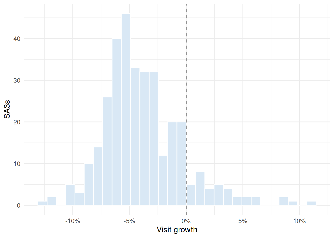
#| fig-cap: "SA3 visit growth from the pre-policy exposure window to clean post-policy quarters."
sa3_growth <- sa3_panel |>
  mutate(window = case_when(
    quarter_date %in% exposure_baseline_quarters$quarter_date ~ "baseline",
    quarter_date >= clean_post_quarter_date ~ "post",
    TRUE ~ NA_character_
  )) |>
  filter(!is.na(window)) |>
  group_by(sa3_key, state, sa3, exposure_band, pre_policy_non_bulk_billed_share, baseline_services, window) |>
  summarise(
    services = mean(services, na.rm = TRUE),
    bb_rate = weighted_rate(bulk_billed_services, services),
    .groups = "drop"
  ) |>
  pivot_wider(names_from = window, values_from = c(services, bb_rate)) |>
  mutate(
    visit_growth = services_post / services_baseline - 1,
    bulk_billing_rate_change = bb_rate_post - bb_rate_baseline,
    exposure_label = as.character(exposure_band)
  ) |>
  filter(is.finite(visit_growth), is.finite(pre_policy_non_bulk_billed_share))

ggplot(sa3_growth, aes(visit_growth)) +
  geom_histogram(bins = 30, fill = "#d9e8f5", colour = "white") +
  geom_vline(xintercept = 0, linetype = "dashed", colour = "grey35") +
  scale_x_continuous(labels = percent) +
  labs(x = "Visit growth", y = "SA3s")
```
```{r}
#| label: exposure-band-trends
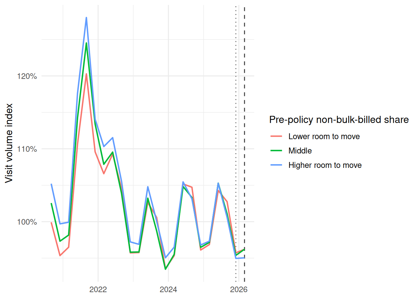
#| fig-cap: "Longer-run quarterly GP visit volume indexed to the four-quarter pre-policy exposure window."
band_trends <- sa3_panel |>
  group_by(exposure_band, quarter_date, quarter_status) |>
  summarise(services = sum(services, na.rm = TRUE), .groups = "drop") |>
  group_by(exposure_band) |>
  mutate(
    baseline_services = mean(services[quarter_date %in% exposure_baseline_quarters$quarter_date], na.rm = TRUE),
    visit_index = services / baseline_services
  ) |>
  ungroup()

ggplot(band_trends, aes(quarter_date, visit_index, colour = exposure_band)) +
  geom_vline(xintercept = transition_quarter_date, linetype = "dotted", colour = "grey45") +
  geom_vline(xintercept = clean_post_quarter_date, linetype = "dashed", colour = "grey25") +
  geom_line(linewidth = 0.8, na.rm = TRUE) +
  scale_y_continuous(labels = percent) +
  labs(x = NULL, y = "Visit volume index", colour = "Pre-policy non-bulk-billed share")
```
The 2021-22 peak is real in the official service counts, not an indexing artefact. It lines up with the pandemic-era disruption and rebound in GP claiming, so it is a poor baseline for the 2025 policy question. The chart below keeps the same index but starts after that shock; the visit-volume models also use this flatter window.
```{r}
#| label: exposure-band-trends-flat-window
#| fig-cap: "Post-spike quarterly GP visit volume indexed to the four-quarter pre-policy exposure window."
band_trends |>
  filter(quarter_date >= visit_model_start_quarter_date) |>
  ggplot(aes(quarter_date, visit_index, colour = exposure_band)) +
  geom_vline(xintercept = transition_quarter_date, linetype = "dotted", colour = "grey45") +
  geom_vline(xintercept = clean_post_quarter_date, linetype = "dashed", colour = "grey25") +
  geom_line(linewidth = 0.8, na.rm = TRUE) +
  scale_y_continuous(labels = percent) +
  labs(x = NULL, y = "Visit volume index", colour = "Pre-policy non-bulk-billed share")
```
```{r}
#| label: exposure-growth-scatter
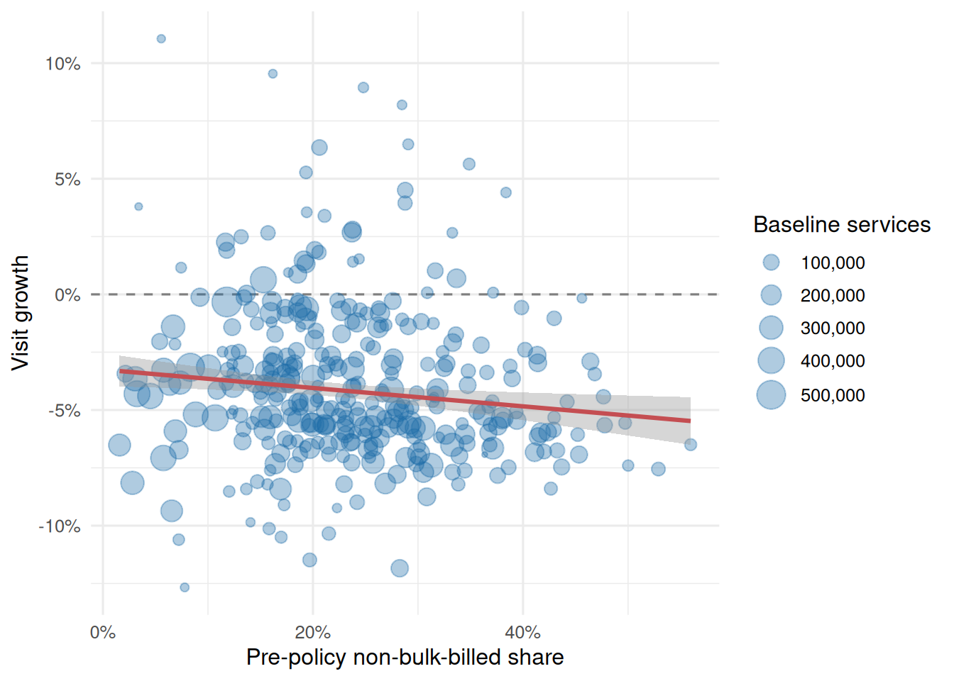
#| fig-cap: "Areas with lower pre-policy bulk billing had more room for the incentives to shift billing behaviour."
ggplot(sa3_growth, aes(pre_policy_non_bulk_billed_share, visit_growth)) +
  geom_hline(yintercept = 0, linetype = "dashed", colour = "grey50") +
  geom_point(aes(size = baseline_services), alpha = 0.35, colour = "#1b6ca8") +
  geom_smooth(aes(weight = baseline_services), method = "lm", se = TRUE, colour = "#c44e52") +
  scale_x_continuous(labels = percent) +
  scale_y_continuous(labels = percent) +
  scale_size_continuous(labels = comma, range = c(1, 7)) +
  labs(
    x = "Pre-policy non-bulk-billed share",
    y = "Visit growth",
    size = "Baseline services"
  )
```
```{r}
#| label: observed-billing-visit-scatter
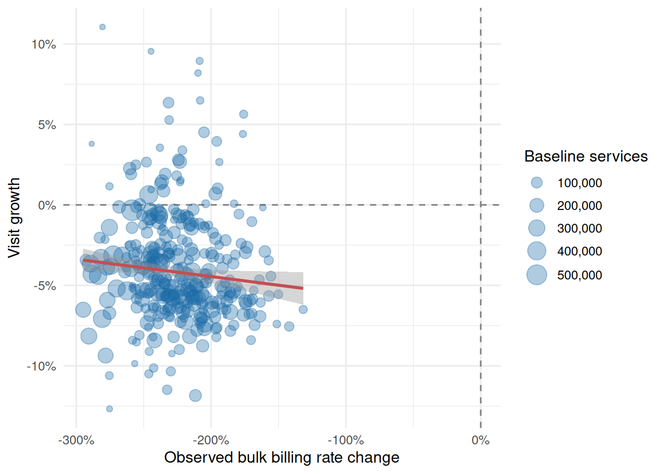
#| fig-cap: "Observed SA3 bulk billing rate change versus visit growth."
ggplot(sa3_growth, aes(bulk_billing_rate_change, visit_growth)) +
  geom_hline(yintercept = 0, linetype = "dashed", colour = "grey50") +
  geom_vline(xintercept = 0, linetype = "dashed", colour = "grey50") +
  geom_point(aes(size = baseline_services), alpha = 0.35, colour = "#1b6ca8") +
  geom_smooth(aes(weight = baseline_services), method = "lm", se = TRUE, colour = "#c44e52") +
  scale_x_continuous(labels = percent) +
  scale_y_continuous(labels = percent) +
  scale_size_continuous(labels = comma, range = c(1, 7)) +
  labs(
    x = "Observed bulk billing rate change",
    y = "Visit growth",
    size = "Baseline services"
  )
```
```{r}
#| label: sa3-access-models
access_model_panel <- sa3_panel |>
  filter(
    quarter_date >= visit_model_start_quarter_date,
    quarter_date != transition_quarter_date
  ) |>
  mutate(post_x_gap_10pp = as.integer(clean_post_policy) * pre_policy_gap_10pp)

fit_access_model <- function(outcome, label, outcome_type) {
  model_data <- access_model_panel |>
    filter(
      is.finite(.data[[outcome]]),
      is.finite(post_x_gap_10pp),
      is.finite(baseline_services),
      baseline_services > 0
    )

  model <- lm(
    reformulate(
      c("factor(sa3_key)", "factor(quarter_date)", "post_x_gap_10pp"),
      response = outcome
    ),
    data = model_data,
    weights = baseline_services
  )

  tidy(model, conf.int = TRUE) |>
    filter(term == "post_x_gap_10pp") |>
    transmute(
      outcome = label,
      interpretation = "Clean post-policy change per 10 percentage point higher pre-policy non-bulk-billed share",
      estimate = format_model_estimate(estimate, outcome_type),
      conf_low = format_model_estimate(conf.low, outcome_type),
      conf_high = format_model_estimate(conf.high, outcome_type),
      rows = nrow(model_data),
      sa3s = n_distinct(model_data$sa3_key)
    )
}

access_model_summary <- bind_rows(
  fit_access_model("log_services", "GP visit volume", "log"),
  fit_access_model("bulk_billing_rate", "Bulk billing rate", "rate"),
  fit_access_model("avg_patient_contribution_patient_billed", "Patient contribution among patient-billed services", "dollar")
)

access_model_summary |> kable()
```
The first row is the key access test. A positive estimate would mean higher-exposure areas had faster visit-volume growth after the clean post-policy quarter. The second and third rows are mechanism checks: the policy story is stronger if the same high-exposure areas also show larger bulk billing rate gains or lower patient contributions.
```{r}
#| label: sa3-event-study
#| fig-cap: "Differential SA3 visit-volume change by pre-policy non-bulk-billed share, relative to September quarter 2025."
reference_quarter <- max(access_model_panel$quarter_date[access_model_panel$quarter_date < transition_quarter_date], na.rm = TRUE)

event_study_data <- access_model_panel |>
  select(sa3_key, quarter_date, log_services, pre_policy_gap_10pp, baseline_services) |>
  left_join(
    access_model_panel |>
      filter(quarter_date == reference_quarter) |>
      select(sa3_key, reference_log_services = log_services),
    by = "sa3_key"
  ) |>
  mutate(delta_log_services = log_services - reference_log_services) |>
  filter(is.finite(delta_log_services), is.finite(pre_policy_gap_10pp), is.finite(baseline_services))

event_study <- event_study_data |>
  group_by(quarter_date) |>
  group_modify(\(.x, .y) {
    tidy(
      lm(delta_log_services ~ pre_policy_gap_10pp, data = .x, weights = baseline_services),
      conf.int = TRUE
    ) |>
      filter(term == "pre_policy_gap_10pp")
  }) |>
  ungroup() |>
  mutate(
    estimate_pct = exp(estimate) - 1,
    conf_low_pct = exp(conf.low) - 1,
    conf_high_pct = exp(conf.high) - 1,
    quarter_status = case_when(
      quarter_date < transition_quarter_date ~ "Pre-policy",
      quarter_date >= clean_post_quarter_date ~ "Clean post-policy",
      TRUE ~ "Transition quarter"
    )
  )

ggplot(event_study, aes(quarter_date, estimate_pct)) +
  geom_hline(yintercept = 0, colour = "grey55") +
  geom_vline(xintercept = transition_quarter_date, linetype = "dotted", colour = "grey45") +
  geom_vline(xintercept = clean_post_quarter_date, linetype = "dashed", colour = "grey25") +
  geom_ribbon(aes(ymin = conf_low_pct, ymax = conf_high_pct), fill = "#d9e8f5", alpha = 0.7) +
  geom_line(colour = "#1b6ca8", linewidth = 0.8) +
  geom_point(aes(shape = quarter_status), colour = "#1b6ca8", size = 2) +
  scale_y_continuous(labels = percent) +
  labs(
    x = NULL,
    y = "Differential visit change per 10pp exposure",
    shape = NULL
  )
```
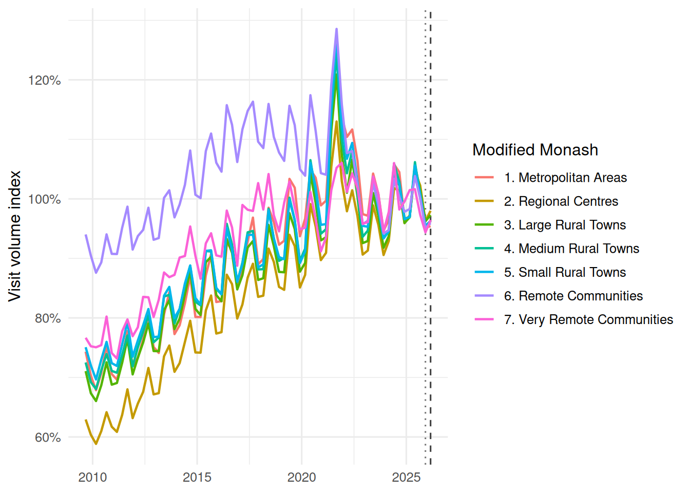
```{r}
#| label: mmm-visit-trends
#| fig-cap: "Modified Monash GP visit volume indexed to the four-quarter pre-policy exposure window."
mmm_trends <- mmm_visits |>
  filter(modified_monash != "Unknown") |>
  group_by(modified_monash, quarter_date, quarter_status) |>
  summarise(services = sum(services, na.rm = TRUE), .groups = "drop") |>
  group_by(modified_monash) |>
  mutate(
    baseline_services = mean(services[quarter_date %in% exposure_baseline_quarters$quarter_date], na.rm = TRUE),
    visit_index = services / baseline_services
  ) |>
  ungroup()

ggplot(mmm_trends, aes(quarter_date, visit_index, colour = modified_monash)) +
  geom_vline(xintercept = transition_quarter_date, linetype = "dotted", colour = "grey45") +
  geom_vline(xintercept = clean_post_quarter_date, linetype = "dashed", colour = "grey25") +
  geom_line(linewidth = 0.8, na.rm = TRUE) +
  scale_y_continuous(labels = percent) +
  labs(x = NULL, y = "Visit volume index", colour = "Modified Monash")
```
```{r}
#| label: unknown-mmm-check
unknown_mmm <- mmm_visits |>
  group_by(quarter, quarter_date) |>
  summarise(
    total_services = sum(services, na.rm = TRUE),
    unknown_services = sum(services[modified_monash == "Unknown"], na.rm = TRUE),
    unknown_share = unknown_services / total_services,
    .groups = "drop"
  ) |>
  filter(quarter_date >= as.Date("2023-09-01")) |>
  arrange(quarter_date)

unknown_mmm |>
  mutate(
    total_services = comma(total_services),
    unknown_services = comma(unknown_services),
    unknown_share = percent(unknown_share, accuracy = 0.001)
  ) |>
  kable()
```
The `Unknown` Modified Monash category is excluded from the indexed MMM chart because it is tiny in absolute terms and appears to have a classification break around the June quarter 2024. It rises from hundreds of services per quarter to roughly 7,000-9,000, but still remains around `r percent(max(unknown_mmm$unknown_share, na.rm = TRUE), accuracy = 0.001)` of GP non-referred attendances. That makes it visually noisy as an index and not a meaningful access geography.
```{r}
#| label: sa3-growth-table
sa3_growth |>
  group_by(exposure_band) |>
  summarise(
    sa3s = n(),
    median_pre_policy_non_bulk_billed_share = median(pre_policy_non_bulk_billed_share, na.rm = TRUE),
    median_visit_growth = median(visit_growth, na.rm = TRUE),
    weighted_visit_growth = weighted.mean(visit_growth, w = baseline_services, na.rm = TRUE),
    .groups = "drop"
  ) |>
  mutate(
    median_pre_policy_non_bulk_billed_share = percent(median_pre_policy_non_bulk_billed_share, accuracy = 0.1),
    median_visit_growth = percent(median_visit_growth, accuracy = 0.1),
    weighted_visit_growth = percent(weighted_visit_growth, accuracy = 0.1)
  ) |>
  kable()
```
## Early Answer
```{r}
#| label: answer-table
national_delta <- window_compare(national)$change[[1]]
age_delta <- window_compare(age_rates) |>
  select(group, change) |>
  arrange(desc(change))
seifa_delta <- window_compare(seifa_rates) |>
  select(group, change) |>
  arrange(desc(change))
visit_access_estimate <- access_model_summary |>
  filter(outcome == "GP visit volume") |>
  pull(estimate) |>
  first()

tibble(
  question = c(
    "Did the national rate move after 1 November 2025?",
    "Was the largest age signal in working-age adults?",
    "Did lower and higher socioeconomic areas both move?",
    "Did higher-exposure SA3s also show more GP visits?",
    "Can we call this access rather than billing?"
  ),
  early_read = c(
    paste0("National before/after change: ", percent(national_delta, accuracy = 0.1), "."),
    paste0("Largest age-band change: ", age_delta$group[[1]], " at ", percent(age_delta$change[[1]], accuracy = 0.1), "."),
    paste0("Largest SEIFA change: ", seifa_delta$group[[1]], " at ", percent(seifa_delta$change[[1]], accuracy = 0.1), "."),
    paste0("SA3 fixed-effects visit estimate: ", visit_access_estimate, " per 10 percentage point higher pre-policy non-bulk-billed share."),
    "Not fully. The data show billing and service-use/payment signals, not unmet need or appointment availability."
  )
) |>
  kable()
```
The early read is that the 1 November 2025 changes should be treated as having shifted measured bulk billing access if the post-November lift is visible nationally, strongest for `16-64`, and not limited to places that already had high bulk billing. The broader access case is stronger if the SA3 visit-volume model shows higher-exposure areas also gaining visits after the clean post-policy quarter. The evidence is weaker if the rise is small relative to normal monthly volatility, if it does not persist in the rolling average, or if service-use checks deteriorate.
## Caveats
- AIHW's monthly dashboard is based on date of service; Department Medicare statistics can differ because official Medicare statistics are generally processed-date based.
- AIHW notes that the last 3 months of monthly dashboard data are preliminary.
- Bulk billing rate is a claim-level access proxy, not a direct measure of unmet need, waiting time or clinic availability.
- The AIHW benefits series excludes Bulk Billing Practice Incentive Program payments.
- LGA statistics are based on patient location. People can travel outside their LGA for care.
- The SA3 visit model uses service counts rather than per-capita rates. SA3 fixed effects absorb stable differences between areas, but population growth can still affect visit volumes.
- The December quarter 2025 is excluded from the visit model because it mixes one pre-policy month with two post-policy months.
- PHN and LGA summaries in this post mix monthly AIHW dashboard data and quarterly Department statistics; they are used as triangulation, not as one single modelled dataset.
- Modified Monash should be added with a proper spatial or fine-geography concordance before making MMM-specific claims.